Swing friction is a term I coined in my PhD thesis and is defined as the differential of swing values between individual performers (or groups of performers). If the swing friction is significantly large and consistently maintained, it may form a characteristic of ensemble feel.
Chuck Berry’s Johnny B. Goode (Berry 1958) provides an instructive example of swing friction. Berry, often considered the father of rock n’ roll, was instrumental in ‘straightening out’ the blues 12/8 shuffle rhythm into the archetypal electric guitar riff. Johnny B. Goode features this ‘straight 8th’ guitar rhythm, as well as equally straight lead playing juxtaposed with a stubbornly bouncy drum, bass and piano feel. Heavily swung quaver values occur in the ride cymbal pattern, often near the 67% mark, a significant deviation of over 52ms from the straight quaver at 170bpm. The guitar rhythm part however remains resolutely straight rarely venturing beyond 52% swing. This already large 15% discrepancy of swing value is exaggerated with the guitar part often sitting on top of the beat (ranging between 0% and -4% latency) leading to a mean separation of about 17% (≈60ms). The lead guitar is equally straight, although not pushed, and occasionally falling behind the beat. Piano interjections are loose but quavers are generally quite swung, mainly in the 60-67% range and repeated quaver triplets prevail. The bass plays mainly crotchets, with the occasional quaver (usually ≈67%). A representative extract from the track can be heard here:
Figure 1 shows a composite two bar template for the lead, rhythm, bass and drum parts, with time-feel components added. There is a huge gap between the swing values of the guitars and bass and drums. The vocal track tends to fall in between these two extremes. In order to hear the effect of swing friction, This example contains electronic sequences of this section with varying time-feel values: 1) as from Figure 1, 2) all instruments at 67% 3) all at 52% 4) all at a middle ground of 60% and 5) back to the ‘true’ values for comparison.
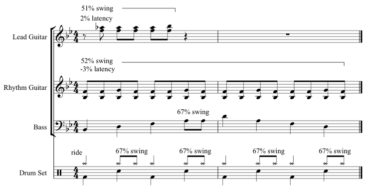
Figure 1. Composite swing and latency values for guitars, bass and drums in Johnny B. Goode.
The sequences have been rendered with MIDI instruments on purpose; although the section would sound better with human performers, but the elimination of the inflection they would inevitably provide allows focus on the power – and limitations – of the SLW model. Mean values for swing and latency have been provided, but the standard deviations of these values introduce the component of looseness or tightness, again different between players. Weighting elements also occur, (the cymbal has a slight emphasis on offbeat quavers for example,) with both mean and standard deviations). This extract plays the sequence first as Figure 1 then with swing, latency, weighting standard deviations from Figure 2 introduced, which add a clearly-defined randomness to each of three time-feel elements, and instruments, individually. There is a subtle but appreciable difference between the sequences; attention to the cymbal pattern, for instance, will reveal a slight offbeat emphasis and looseness.
| Lead Guitar | Rhythm Guitar | Bass | Drums |
| µs= 51 ∂s=1.5 µl= 2 ∂l=
µw= -3 ∂w= 2 |
µs= 52 ∂s=1
µl= -3 ∂l= 1 µw= -3 ∂w= 2 |
µs= 67 ∂s=2
µl= 0 ∂l= 1 µw= 4 ∂w= 2 |
µs= 67 ∂s=2
µl= 0 ∂l= 0 µw= 2 ∂w= 1 |
Figure 2 Mean and standard deviation values of swing, latency and
weighting (measured as dB level)
An averaging out of time-feel components over the entire track runs the risk of over-generalization and may incorrectly group specific mechanisms that occur only occasionally. There are for example, brief moments when the bass seems to join with the rhythm guitar’s straight quavers. There is also the assumption, with a single matrix per instrument, that all beats of the bar are the same, which ignores the emphasis on crotchets 2 and 4 in the drums. Matrices could be provided for beats 1 and 2, and beats 3 and 4 separately, or even weighting at the crotchet level, for greater sophistication when needed.
Despite these acknowledged limitations, the discretionary use of this type of analysis allows for an instructive and parsimonious description of ensemble time-feel elements.

7 replies on “Swing Friction in Johnny B. Goode”
Hi, this is fascinating. What kind of software do you use for these exact mathematical analyses?
Thanks Ralf. In the absence of multitracks it was neither automatic nor definitive. But essentially I used transient detection on a sonogram in various frequency bands (audiosculpt I think? It was back in 2008), then (as explained in my thesis) used simple maths to calculate swing and latency values. These gave me timings that I could put in MIDI (Logic Pro) to check against the original. I checked informally with various percussion colleagues on the ‘feel’. and made the rudimentary MIDI realisations. I think that the straight guitar vs swung rhythm section concept is (for me) extremely convincing although readily accept the limitations (and usefulness) of minute gradations.
Thanks for sharing this! I’m not able to listen to the audio clips, even after updating flash. (in chrome, a message says to update flash player, even immediately after update) Would love to hear them though!
Apologies. Could you try now?
It works!
As I listened to Johnny B Goode and noticed the swing drums vs the straight guitar, I thought my ears must be deceiving me, but then I found your article which confirmed my impression. It’s very interesting work and it has made me rethink what I thought I knew about timing; thank you for sharing it.
[…] “Swing Friction in Johnny B. Goode”. Miltonline. March 19, 2017. Retrieved August 15, 2024. […]